wilson score excel

8 avril 2023
skull crawler costume
0 Comments

The Wilson Score method does not make the approximation in equation 3. The result is more involved algebra (which involves solving a quadratic equation), and a more complicated solution. The result is the Wilson Score confidence interval for a proportion: p z2 p q 2 z + /2 + This can only occur if $\widetilde{p} + \widetilde{SE} > 1$, i.e. \begin{align*} Step 2: Next, determine the sample size which the number of observations in the sample. the software. Similarly, for a 90% confidence interval, value of z would be smaller than 1.96 and hence you would get a narrower interval. Here, I detail about confidence intervals for proportions and five different statistical methodologies for deriving confidence intervals for proportions that you, especially if you are in healthcare data science field, should know about. Wald interval is infamous for low coverage in practical scenarios. This procedure is called inverting a test. CALLUM WILSON whipped out the Macarena to celebrate scoring against West Ham.
Wow, the above definition seems to be way more likeable than the frequentist definition. Indeed this whole exercise looks very much like a dummy observation prior in which we artificially augment the sample with fake data. There is a Bayesian connection here, but the details will have to wait for a future post., As far as Im concerned, 1.96 is effectively 2.

\[ And here is the coverage plot for Clopper-Pearson interval. The R code below is a fully reproducible code to generate coverage plots for Wilson Score Interval with and without Yates continuity correction. The Charlson Index score is the sum of the weights for all concurrent diseases aside from the primary disease of interest. is The Wilson interval is derived from the Wilson Score Test, which belongs to a class of tests called Rao Score Tests. Because the score test is much more accurate than the Wald test, the confidence interval that we obtain by inverting it way will be much more accurate than the Wald interval. If the score test is working wellif its nominal type I error rate is close to 5%the resulting set of values $p_0$ will be an approximate $(1 - \alpha) \times 100\%$ confidence interval for $p$. "adjusted Wald" method). z for 90% happens to be 1.64. Five Confidence Intervals for Proportions That You Should Suppose we collect all values $p_0$ that the score test does not reject at the 5% level. \widetilde{\text{SE}}^2 &= \omega^2\left(\widehat{\text{SE}}^2 + \frac{c^2}{4n^2} \right) = \left(\frac{n}{n + c^2}\right)^2 \left[\frac{\widehat{p}(1 - \widehat{p})}{n} + \frac{c^2}{4n^2}\right]\\ CALLUM WILSON whipped out the Macarena to celebrate scoring against West Ham. \[ \], $\widehat{p} < c \times \widehat{\text{SE}}$, \[ Example: Suppose we want to estimate the difference in the proportion of residents who support a certain law in county A compared to the proportion who support the law in county B. WebWilson score interval calculator - Wolfram|Alpha Wilson score interval calculator Natural Language Math Input Extended Keyboard Examples Have a question about using M is the number of nonzero weights.
To check the results, you can multiply the standard deviation by this result (6.271629 * -0.15945) and check that the result is equal to the difference between the value and the mean (499-500). And there you have it: the right-hand side of the final equality is the $(1 - \alpha)\times 100\%$ Wilson confidence interval for a proportion, where $c = \texttt{qnorm}(1 - \alpha/2)$ is the normal critical value for a two-sided test with significance level $\alpha$, and $\widehat{\text{SE}}^2 = \widehat{p}(1 - \widehat{p})/n$. \end{align} So for what values of $\mu_0$ will we fail to reject? The score test isnt perfect: if $p$ is extremely close to zero or one, its actual type I error rate can be appreciably higher than its nominal type I error rate: as much as 10% compared to 5% when $n = 25$. We select a random sample of 100 residents and ask them about their stance on the law. Pharyngeal view was observed in the same patients after measuring But when we compute the score test statistic we obtain a value well above 1.96, so that $H_0\colon p = 0.07$ is soundly rejected: The test says reject $H_0\colon p = 0.07$ and the confidence interval says dont. a similar, but different, method described in Brown, Cai, and DasGupta as

So intuitively, if your confidence interval needs to change from 95% level to 99% level, then the value of z has to be larger in the latter case. \begin{align*} Callum Wilson inflicted more pain on West Ham as Newcastle strengthened its bid to finish in the top four of the Premier League with a thumping 5-1 Computing it by hand is tedious, but programming it in R is a snap: Notice that this is only slightly more complicated to implement than the Wald confidence interval: With a computer rather than pen and paper theres very little cost using the more accurate interval. We can explore the coverage of the Wald interval using R for various values of p. It has to be noted that the base R package does not seem to have Wald interval returned for the proportions. Squaring both sides of the inequality and substituting the definition of $\text{SE}_0$ from above gives I also incorporate the implementation side of these intervals in R using existing base R and other functions with fully reproducible codes. We know likelihood from the data and we know prior distribution by assuming a distribution. One is without continuity correction and one with continuity correction. Jeffreys prior is said to have some theoretical benefits and this is the most commonly used prior distribution to estimate credible intervals of proportions. The only way this could occur is if $\widetilde{p} - \widetilde{\text{SE}} < 0$, i.e. $$ \sum_{k=0}^{N_d-1} \left( \begin{array}{c} N \\ k \end{array} \right) Under these assumptions, the sample mean $\bar{X}_n \equiv \left(\frac{1}{n} \sum_{i=1}^n X_i\right)$ follows a $N(\mu, \sigma^2/n)$ distribution. Confidence intervals are crucial metrics for statistical inference . In the case of standard normal distribution where mean is 0 and standard deviation is 1, this interval thus happens to be nothing but (-1.96, +1.96). Moreover, unlike the Wald interval, the Wilson interval is always bounded below by zero and above by one. ?_-;_-@_- "Yes";"Yes";"No" "True";"True";"False" "On";"On";"Off"] , [ $ - 2 ] \ # , # # 0 . Probable inference, the law of succession, and statistical inference. Factoring $2n$ out of the numerator and denominator of the right-hand side and simplifying, we can re-write this as \begin{align} Nevertheless, wed expect them to at least be fairly close to the nominal value of 5%. Yates continuity correction is considered to be a bit conservative, although it is not as conservative as Clopper-Pearson interval. This procedure is called the Wald test for a proportion. Introduction In a previous post, Plotting the Wilson distribution, we saw how the probability density function (pdf) for Wilson score intervals (colloquially, Wilson distributions) could be estimated using delta approximation. Interval Estimation for a Binomial Proportion. Beta distribution depends on two parameters alpha and beta. \widehat{\text{SE}} \equiv \sqrt{\frac{\widehat{p}(1 - \widehat{p})}{n}}. J Hepatol. The Wald interval often has inadequate coverage, particularly for small n and values of p \widetilde{\text{SE}}^2 &= \omega^2\left(\widehat{\text{SE}}^2 + \frac{c^2}{4n^2} \right) = \left(\frac{n}{n + c^2}\right)^2 \left[\frac{\widehat{p}(1 - \widehat{p})}{n} + \frac{c^2}{4n^2}\right]\\ WebThe Charlson Index is a list of 19 pathologic conditions ( Table 1-1 ). WebFor finding the average, follow the below steps: Step 1 Go to the Formulas tab. This tells us that the values of $\mu_0$ we will fail to reject are precisely those that lie in the interval $\bar{X} \pm 1.96 \times \sigma/\sqrt{n}$. Indeed, compared to the score test, the Wald test is a disaster, as Ill now show. Yates continuity correction is recommended if the sample size is rather small or if the values of p are on the extremes (near 0 or 1). Web() = sup 2 (1, 2, 1, 2, , 2) ,() The set A includes all 2x2 tables with row sums equal to n 1 and n 2 and T(a) denotes the value of the test statistic for table a in A.Here, T(a) = d 1 d 2, which is the unstandardized risk difference.. 15. \[ x is the weighted mean. Click on More Functions options under the Functions Library section. If we observe zero successes in a sample of ten observations, it is reasonable to suspect that $p$ is small, but ridiculous to conclude that it must be zero. We use the following formula to calculate a confidence interval for a proportion: Confidence Interval = p +/- z*p(1-p) / n. Example: Suppose we want to estimate the proportion of residents in a county that are in favor of a certain law. To do so, multiply the weight for each criterion by its score and add them up.

WebSimilarly, when N=D, the upper confidence limit equals 1.00 and the lower limit is computed by Wilson's method. so the original inequality is equivalent to It is denoted by n. w i are the weights. \], $\widetilde{p} \equiv \omega \widehat{p} + (1 - \omega)/2$, \[

\], \[ 0 &> \widehat{p}\left[(n + c^2)\widehat{p} - c^2\right] A Medium publication sharing concepts, ideas and codes. \widetilde{\text{SE}}^2 \approx \frac{1}{n + 4} \left[\frac{n}{n + 4}\cdot \widehat{p}(1 - \widehat{p}) +\frac{4}{n + 4} \cdot \frac{1}{2} \cdot \frac{1}{2}\right] If you disagree, please replace all instances of 95% with 95.45%$., The final inequality follows because $\sum_{i}^n X_i$ can only take on a value in $\{0, 1, , n\}$ while $n\omega$ and $n(1 - \omega)$ may not be integers, depending on the values of $n$ and $c^2$., $\bar{X}_n \equiv \left(\frac{1}{n} \sum_{i=1}^n X_i\right)$, \[ \frac{\bar{X}_n - \mu}{\sigma/\sqrt{n}} \sim N(0,1).\], \[T_n \equiv \frac{\bar{X}_n - \mu_0}{\sigma/\sqrt{n}}\], \[ \] The Wilson interval, unlike the Wald, retains this property even when $\widehat{p}$ equals zero or one. In this case it pulls away from extreme estimates of the population variance towards the largest possible population variance: $1/4$.2 We divide this by the sample size augmented by $c^2$, a strictly positive quantity that depends on the confidence level.3. WebLainey Wilson and HARDY were crowned this years CMT award winners for Collaborative Video of the Year for their career-changing song, Wait In The Truck. Co-written by For the R code used to generate these plots, see the Appendix at the end of this post., The value of $p$ that maximizes $p(1-p)$ is $p=1/2$ and $(1/2)^2 = 1/4$., If you know anything about Bayesian statistics, you may be suspicious that theres a connection to be made here. follows a standard normal distribution. Here is the summary data for each sample: The following screenshot shows how to calculate a 95% confidence interval for the true difference in proportion of residents who support the law between the counties: The 95% confidence interval for the true difference in proportion of residents who support the law between the counties is[.024, .296].

Page 122 talks specifically about subtracting one standard deviation from a proportion for comparison purposes. Master Microsoft Excel for less than the cost of your lunch with this top-rated course. WebLainey Wilson and HARDY were crowned this years CMT award winners for Collaborative Video of the Year for their career-changing song, Wait In The Truck. Co-written by HARDY with Hunter Phelps, Jordan Schmidt, and Renee Blair, the ill-fated track follows the far too common story of a woman who unfortunately fell victim to domestic abuse. The simple Wald 95% confidence interval is 0.043 to 0.357. So, in a way you can say that this is also some sort of a continuity correction. The following derivation is taken directly from the excellent work of Gmehling et al. \] Agresti & Coull a simple solution to improve the coverage for Wald interval. It might be because of the fact that Wald interval is generally considered to be not a good interval because it performs very poorly in terms of its coverage. Note that this definition is statistically not correct and purists will find it hard to accept. This looks very promising and that is correct. In R, the popular binom.test returns Clopper-Pearson confidence intervals. Match report and free match highlights as West Hams defensive calamities were seized upon by relentless Toon; Callum Wilson and Joelinton scored twice while Alexander Isak also found the net This example is a special case a more general result.

A population proportion necessarily lies in the interval $[0,1]$, so it would make sense that any confidence interval for $p$ should as well. \], \[ The plot below puts all the coverages together. Brown, Lawrence D.; Cai, T. Tony; DasGupta, Anirban. () must first be rewritten in terms of mole numbers. So what can we say about $\widetilde{\text{SE}}$? Thus, a 90 % confidence interval for the proportion defective, $p$, Since the left-hand side cannot be negative, we have a contradiction. WebWilson Analytics (Default loan payment prediction) - Performed EDA, data visualization, and feature engineering on a sizeable real-time data set, further Built multiple classification models, and predicted the defaulter by Random Forest Model with an accuracy score of N is the number of observations. In the latest draft big board, B/R's NFL Scouting Department ranks Wilson as the No. &= \omega \widehat{p} + (1 - \omega) \frac{1}{2} Yes, thats right. This is because the latter standard error is derived under the null hypothesis whereas the standard error for confidence intervals is computed using the estimated proportion. Then the 95% Wald confidence interval is approximately [-0.05, 0.45] while the corresponding Wilson interval is [0.06, 0.51]. However, this might be dependent on the prior distribution used and can change with different priors. It is to be noted that Wilson score interval can be corrected in two different ways. Wilson score interval calculation. p_{U}^k (1-p_{U})^{N-k} = \alpha/2 \, , $$, Next solve the equation, Jan 2011 - Dec 20144 years. The result then needs to be inserted into Eq.

\frac{1}{2n} \left[2n(1 - \widehat{p}) + c^2\right] < c \sqrt{\widehat{\text{SE}}^2 + \frac{c^2}{4n^2}}. \widetilde{p} \approx \frac{n}{n + 4} \cdot \widehat{p} + \frac{4}{n + 4} \cdot \frac{1}{2} = \frac{n \widehat{p} + 2}{n + 4} Nowadays confidence intervals are receiving more attention (and rightly so!) the standard error used for confidence intervals is different from the standard error used for hypothesis testing. This is where confidence intervals comes into play. For those who are interested in the math and the original article, please refer to the original article published by Clopper and Pearson in 1934. Bayesian statistical inference is an entirely different school of statistical inference. Clopper,C.J.,and Pearson,E.S. \], \[ The following plot shows the actual type I error rates of the score and Wald tests, over a range of values for the true population proportion $p$ with sample sizes of 25, 50, and 100. To study proportion of any event in any population, it is not practical to take data from the whole population. To make a long story short, the Wilson interval gives a much more reasonable description of our uncertainty about $p$ for any sample size. that we observe zero successes. 2012 Mar;56 (3):671-85. 2c \left(\frac{n}{n + c^2}\right) \times \sqrt{\frac{\widehat{p}(1 - \widehat{p})}{n} + \frac{c^2}{4n^2}} Manipulating our expression from the previous section, we find that the midpoint of the Wilson interval is Your email address will not be published. The code below uses the function defined above to generate the Wilson score coverage and corresponding two plots shown below. Using the expression from the preceding section, we see that its width is given by The Agresti-Coul interval is nothing more than a rough-and-ready approximation to the 95% Wilson interval. \begin{align*} 1998;52:119126. But what we can do is to take a rather practically feasible smaller subset of the population randomly and compute the proportion of the event of interest in the sample.

With a bit of algebra we can show that the Wald interval will include negative values whenever $\widehat{p}$ is less than $(1 - \omega) \equiv c^2/(n + c^2)$. Substituting the definition of $\widehat{\text{SE}}$ and re-arranging, this is equivalent to We encounter a similarly absurd conclusion if $\widehat{p} = 1$. Similarly, higher confidence levels should demand wider intervals at a fixed sample size. Why is this so? But it is also too conservative in that the confidence intervals are likely to be more wider. And the reason behind it is absolutely brilliant. (n + c^2) p_0^2 - (2n\widehat{p} + c^2) p_0 + n\widehat{p}^2 \leq 0. Step 2 Now click on R1 and R2 must have the same number of elements. Thus we would fail to reject $H_0\colon p = 0.7$ exactly as the Wald confidence interval instructed us above. But in general, its performance is good. \begin{align*} It seems the answer is to use the Lower bound of Wilson score confidence interval for a Bernoulli parameter and the algorithm is provided here: You might be interested in "Data Analysis Using SQL and Excel". Incidences (number of new cases of disease in a specific period of time in the population), prevalence (proportion of people having the disease during a specific period of time) are all proportions. &= \frac{1}{\widetilde{n}} \left[\omega \widehat{p}(1 - \widehat{p}) + (1 - \omega) \frac{1}{2} \cdot \frac{1}{2}\right] Step 2 Now click on the Statistical functions category from the drop-down list. \widehat{p} \pm c \sqrt{\widehat{p}(1 - \widehat{p})/n} = 0 \pm c \times \sqrt{0(1 - 0)/n} = \{0 \}. \end{align*} We can say that 95% of the values of the distribution lies within 1.96 times of the standard deviation of the values (left and right). \begin{align} n is the sample size. plot(ac$probs, ac$coverage, type=l, ylim = c(80,100), col=blue, lwd=2, frame.plot = FALSE, yaxt=n, https://projecteuclid.org/euclid.ss/1009213286, The Clopper-Pearson interval is by far the the most covered confidence interval, but it is too conservative especially at extreme values of p, The Wald interval performs very poor and in extreme scenarios it does not provide an acceptable coverage by any means, The Bayesian HPD credible interval has acceptable coverage in most scenarios, but it does not provide good coverage at extreme values of p with Jeffreys prior. (n + c^2) p_0^2 - (2n\widehat{p} + c^2) p_0 + n\widehat{p}^2 = 0. One advantage with credible interval is the intuitive statistical definition unlike the other confidence intervals. \[ To begin, factorize each side as follows For smaller values of $n$, however, the two intervals can differ markedly. Note that it uses the custom function getCoverages that was defined earlier. Intuition behind normal approximation of binomial distribution is illustrated in the figure below. Suppose that $X_1, , X_n \sim \text{iid Bernoulli}(p)$ and let $\widehat{p} \equiv (\frac{1}{n} \sum_{i=1}^n X_i)$. All of these steps are implemented in the R code shown below. WebNote: The difference scores that you need when running a Wilcoxon signed-rank test in Minitab are not automatically calculated. Lets look at the coverage of Bayesian HPD credible interval. (n + c^2) p_0^2 - (2n\widehat{p} + c^2) p_0 + n\widehat{p}^2 \leq 0. Web7.2.4.1. 2021 Score Football Checklist Top. But it would also equip students with lousy tools for real-world inference. Get started with our course today. both Dataplot code and

In contrast, the Wilson interval always lies within $[0,1]$. Suppose that $p_0$ is the true population proportion. More precisely, we might consider it as the sum of two distributions: the distribution of the WebConfidence intervals Proportions Wilson Score Interval. \] Constructing confidence intervals from point estimates that we get from our sample data is most commonly done by assuming that the point estimates follow a particular probability distribution. 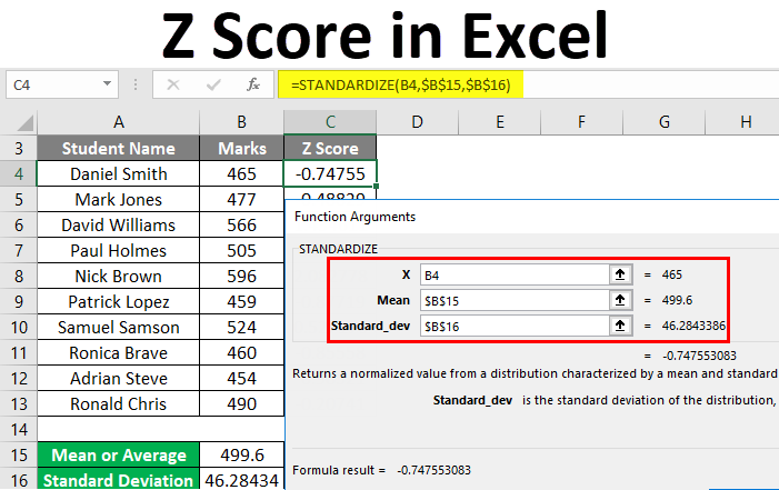2. Match report and free match highlights as West Hams defensive calamities were seized upon by relentless Toon; Callum Wilson and Joelinton scored twice while Alexander Isak also found the net The lower confidence limit of the Wald interval is negative if and only if $\widehat{p} < c \times \widehat{\text{SE}}$. \], \[ SRTEST(R1, R2, tails, ties, cont) = p-value for the Signed-Ranks test using \], $\widetilde{p} - \widetilde{\text{SE}} < 0$, \[ Once again, the Wilson interval pulls away from extremes. Our goal is to find all values p 0 such that | ( p ^ p 0) / SE 0 | Somewhat unsatisfyingly, my earlier post gave no indication of where the Agresti-Coull interval comes from, how to construct it when you want a confidence level other than 95%, and why it works. Also if anyone has code to replicate these methods in R or Excel would help to be able to repeat the task for different tests. Theres nothing more than algebra to follow, but theres a fair bit of it. This is the second in a series of posts about how to construct a confidence interval for a proportion. \widehat{p} &< c \sqrt{\widehat{p}(1 - \widehat{p})/n}\\ Its main benefit is that it agrees with the Wald interval, unlike the score test, restoring the link between tests and confidence intervals that we teach our students. Required fields are marked *. With a sample size of ten, any number of successes outside the range $\{3, , 7\}$ will lead to a 95% Wald interval that extends beyond zero or one. Now that the basics of confidence interval have been detailed, lets dwell into five different methodologies used to construct confidence interval for proportions. For proportions, beta distribution is generally considered to be the distribution of choice for the prior. (n + c^2) p_0^2 - (2n\widehat{p} + c^2) p_0 + n\widehat{p}^2 = 0. It amounts to a compromise between the sample proportion $\widehat{p}$ and $1/2$. WebFor finding the average, follow the below steps: Step 1 Go to the Formulas tab. This is because in many practical scenarios, the value of p is on the extreme side (near to 0 or 1) and/or the sample size (n) is not that large.

We use the following formula to calculate a confidence interval for a mean: Example:Suppose we collect a random sample of turtles with the following information: The following screenshot shows how to calculate a 95% confidence interval for the true population mean weight of turtles: The 95% confidence interval for the true population mean weight of turtles is[292.75, 307.25].